7.3 Cournot's duopoly model
Model
One model of duopoly is the strategic game in which- the players are the firms
- the actions of each firm are the set of possible outputs (any nonnegative amount)
- the payoff of each firm is its profit.
This game models a situation in which each firm chooses its output independently, and the market determines the price at which it is sold. Specifically, if firm 1 produces the output y1 and firm 2 produces the output y2 then the price at which each unit of output is sold is P(y1 + y2), where P is the inverse demand function.
Denote firm 1's total cost function by TC1(y) and firm 2's by TC2(y). Then firm 1's total revenue when the pair of outputs chosen by the firms is (y1, y2) is P(y1 + y2)y1, so that its profit is
The solution we apply to this game is that of Nash equilibrium. To think about the Nash equilibria, first consider the nature of the firms' best response functions.
The firms' best response functions
Firm 1's best response function gives, for each possible output of firm 2, the profit-maximizing output of firm 1. Firm 1's profit-maximizing output when firm 2's output is y2 is the output y1 that maximizes firm 1's profit; that is, the value of y1 that maximizesP(y1 + y2)y1 − TC1(y1).Differentiating with respect to y1 (treating y2 as a constant), we conclude that the profit-maximizing output y1 satisfies
P'(y1 + y2)y1 + P(y1 + y2) − MC1(y1) = 0.
We'd like to know the shape of firm 1's best response function—i.e. we'd like to know how the value of y1 that satisfies this condition depends on y2.
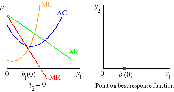
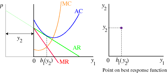
Consider a case in which firm 1's average cost function takes the "typical" U shape. First suppose that y2 = 0. Then firm 1's problem is the same as that of a monopolist. Its best output satisfies the condition MR = MC1, as illustrated in the left panel of the following figure. The corresponding point on firm 1's best response function is shown in the right panel: when y2 = 0, firm 1's best output is b1(0).
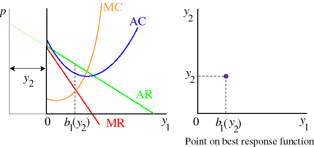
Now increase y2. Firm 2 now absorbs some of the demand, and less is left over for firm 1: the demand curve firm 1 faces is shifted to the left by the amount y2, as in the left panel of the following figure. Firm 1's best output satisfies the condition that its marginal revenue, given the part of the demand function that it faces, is equal to its marginal cost. This optimal output is indicated as b1(y2) in the left panel of the figure; the corresponding point on firm 1's best response function is shown in the right panel.
As firm 2's output increases, there comes a point where there is no positive output at which firm 1 can make a profit. The critical point is shown in the left panel of the following figure. In this case, the most profit firm 1 can earn by producing a positive output is 0: the AR curve it faces is tangent to its AC curve. The corresponding point on firm 1's best response function is shown in the right panel.
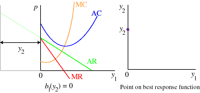
For larger outputs, firm 1's optimal output is zero, as shown in the following figure.
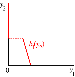
Firm 1's whole best response function is shown in the following figure. The way to read this figure is to take a point on the vertical axis—a value of y2—and go across to the graph, then down to the horizontal axis; the value of y1 on this axis is firm 1's optimal output given y2.
If firm 2's cost function is the same as firm 1's, then its best response function is symmetric with firm 1's, as shown in the following figure.
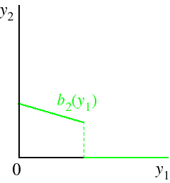
Whenever a firm's average cost functions is U-shaped, its best response function has a "jump" in it, for the same reason that a competitive firm's supply function has a "jump" in it: the firm either wants to produce outputs close to its efficient scale of production or it wants to produce an output of zero, but it does not want to produce intermediate outputs (for which the average cost is high).
A firm's best output does not necessarily decrease as its rival's output increases. Such a relationship seems likely, though it is possible that for some increases in its rival's output, a firm wants to produce more output, not less.
Nash equilibrium
To find a Nash equilibrium, we need to put together the two best response functions. Any pair (y1, y2) of outputs at which they intersect has the property thatThe best response functions are superimposed in the following figure.
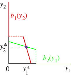
We see that for this pair of best response functions there is a unique Nash equilibrium, indicated by the small purple disk. (In general, there may be more than one Nash equilibrium.)
To find a Nash equilibrium of Cournot's model for a specific cost function and demand function we follow the general procedure for finding a Nash equilibrium of a game using best response functions.
- Example
-
Each of two firms has the cost function TC(y) = 30y; the inverse demand function for the firms' output is p = 120 − Q, where Q is the total output. What are the firms' outputs in a Nash equilibrium of Cournot's model?
- First find the firms' best response functions. Firm 1's profit is
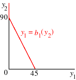
y1(120 − y1 − y2) − 30y1.Taking the derivative of this profit with respect to y1 (holding y2 constant) and setting the derivative equal to zero we obtain120 − 2y1 − y2 − 30 = 0,ory1 = (90 − y2)/2.Thus the best response function of firm 1 is given by b1(y2) = (90 − y2)/2. This function is shown in the following figure.
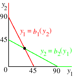
Similarly, we find that the best response function of firm 2 is given by b2(y1) = (90 − y1)/2. This function is superimposed on the best response function of firm 1 in the following figure.
- We now need to find a pair (y1, y2) of outputs with the property that
y1 = b1(y2) and y2 = b2(y1).That is,y1 = (90 − y2)/2 and y2 = (90 − y1)/2.Substituting one equation in the other we obtain y1 = (90 − (90 − y1)/2)/2, so that y1 = 30; substituting in the equation for y2 we get y2 = 30.
- First find the firms' best response functions. Firm 1's profit is
- Example
-
Each of two firms has the cost function TC(y) = y2. As in the previous example, the inverse demand function for the firms' output is p = 120 − Q, where Q is the total output. What are the firms' outputs in a Nash equilibrium of Cournot's model?
- First find the firms' best response functions. If firm 1 chooses the output y1 its profit is
y1(120 − y1 − y2) − y2Taking the derivative of this profit with respect to y1 (holding y2 constant) and setting the derivative equal to zero we obtain
1.120 − 2y1 − y2 − 2y1 = 0,ory1 = (120 − y2)/4.Thus the best response function of firm 1 is given by b1(y2) = (120 − y2)/4.Similarly, we find that the best response function of firm 2 is given by b2(y1) = (120 − y1)/4.
- We now need to find a pair (y1, y2) of outputs with the property that
y1 = b1(y2) and y2 = b2(y1).That is,y1 = (120 − y2)/4 and y2 = (120 − y1)/4.Substituting one equation in the other we obtain y1 = (120 − (120 − y1)/4)/4, so that y1 = 24; substituting in the equation for y2 we get y2 = 24.
- First find the firms' best response functions. If firm 1 chooses the output y1 its profit is
Comparison with competitive equilibrium
In a Nash equilibrium, each firm's output maximizes its profit given the output of the other firm. As we saw above, this implies that for a Nash equilibrium (y*1, y*2), firm 1's output y*1 satisfiesWe conclude that the firms' outputs and the price are different in a Nash equilibrium than they are in a competitive equilibrium. If P'(y*1 + y*2) < 0, as we should expect (the demand curve slopes down), price exceeds marginal cost, so that, as for a monopoly, the total output produced by the firms is less than the competitive output.
An implication is that, as for a monopoly, the Nash equilibrium outcome in a Cournot duopoly is not Pareto stable.
Comparison with monopoly equilibrium
Let (y*1, y*2) be a Nash equilibrium, and consider the pairs (y1, y2) of outputs that yield firm 1 the same profit as it obtains in the equilibrium. The set of such pairs is known as an isoprofit curve of firm 1.In the equilibrium, firm 1's profit is maximal, given firm 2's output y*2. Further, for smaller outputs of firm 2, firm 1's maximal profit is higher (when firm 2 produces less, more of the market is left over for firm 2). In fact, for any given output y2 < y*2 of firm 2, there is a range of outputs close to y*1 for which firm 1's profit exceeds its equilibrium profit. Thus firm 1's isoprofit curve corresponding to the profit it makes in an equilibrium has the shape of the red curve in the following figure.
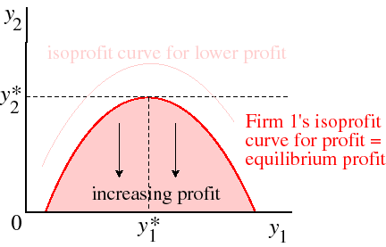
The pink shaded area in this figure is the set of pairs (y1, y2) of outputs that yield firm 1 more profit than does the equilibrium (y*1, y*2). (Firm 1 is better off, given output y1, the lower is firm 2's output—since as firm 2's output decreases, the price increases.)
Now consider the analogous isoprofit curve for firm 2: the set of all pairs (y1, y2) of outputs that yield firm 2 the same profit as it obtains in the equilibrium. This curve is shown in the following figure.
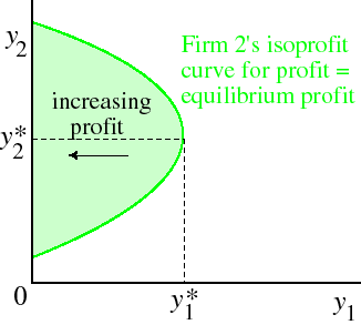
If we put the two curves in the same figure we obtain the following figure.
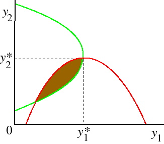
The lens-shaped area shaded brown is the set of pairs (y1, y2) of outputs for which both firms' profits are higher than they are in equilibrium. So long as the isoprofit curves are smooth, this area always exists. That is:
The pair of Nash equilibrium outputs for the firms in Cournot's model does not maximize the firms' total profit. In particular, the total output of the firms in a Nash equilibrium is different from the monopoly output.
- Example
-
Each of two firms has the cost function TC(y) = 30y; the inverse demand function for the firms' output is p = 120 − Q, where Q is the total output. Compare the Nash equilibrium of Cournot's model with the competitive outcome and the monopoly outcome.
We know that in the unique Nash equilibrium each firm's output is 30.
In a long run competitive equilibrium the price is equal to the minimum average cost, which is 30. Thus the total output of the firms is Q such that 30 = 120 − Q, or Q = 90.
A monopolist chooses the output for which MC is equal to MR. We have TR(y) = y(120 − y), so MR(y) = 120 − 2y. Thus the monopolist's output y satisfies MC(y) = 30 = 120 − 2y, or y = 45.
In summary, the three outcomes are given in the following table.
Total output Price Competition 90 30 Duopoly 60 60 Monopoly 45 75
