6.1 Profit-maximizing monopolist setting a single price
Basic theory
A firm is a monopolist if it has no close competitors, and hence can ignore the potential reactions of other firms when choosing its output and price.Theory: a monopolist chooses its output to maximize its profit, given the relationship between output and price as embodied in the aggregate demand function for the good it sells.
Denote by TC the monopolist's total cost function, and by TR its total revenue function (that is, TR is the product of the firm's output and the price that output fetches, given the demand function). Then the monopolist's profit is
Finally, the monopolist's profit at y* must be nonnegative (in the long run), otherwise it would not stay in business.
In summary:
The profit maximizing output y* of a monopolist is either 0 or is positive and satisfies the following conditions:
- MR(y*) = MC(y*)
- MR'(y*) ≤ MC'(y*)
- π(y*) ≥ 0.
Marginal revenue and the demand function
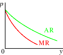
Denote the inverse demand function by P(y). (That is, for any output y, P(y) is the price such that the aggregate demand at p is equal to y.)The monopolist's total revenue is TR(y) = yP(y), so its marginal revenue function is given by

(AR and MR are related in the same way that any average and marginal curves are related.)
Marginal revenue and the elasticity of demand
The price elasticity of demand is defined by- MR(y) > 0 if |η(y)| > 1 (demand is elastic)
- MR(y) < 0 if |η(y)| < 1 (demand is inelastic).
- Example
-
Suppose the demand curve is linear, given by P(y) = a − by (where a and b are constants). Then
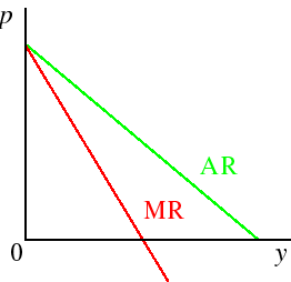
TR(y) = yP(y) = ay − by2,soMR(y) = a − 2by.These functions are shown in the following figure.
- Example
-
Suppose the demand curve is given by P(y) = a/y (where a is a constant). Then
TR(y) = yP(y) = a,so MR(y) = 0. That is, the revenue obtained from selling an extra unit is zero: the price goes down enough to cancel out any gain.
- Example
-
Suppose the demand curve is given by P(y) = a/y2 (where a is a constant). Then
TR(y) = yP(y) = a/y,soMR(y) = −a/y2.That is, the revenue obtained from selling an extra unit is negative: the price goes down enough to cause an increase in volume to lead to a decrease in revenue.
Graphical representation of conditions for profit-maximization
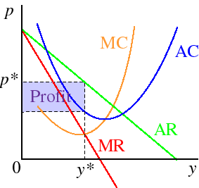
For a downward-sloping linear inverse demand (average revenue) curve, the conditions satisfied by a positive profit maximizing output are represented in the following figure.

The three conditions that any positive optimal output y* must satisfy correspond to the following three properties of the curves in the figure.
- MR(y*) = MC(y*):
- The output y* is determined by the intersection of the MR and MC curves.
- MR'(y*) ≤ MC'(y*):
- At the intersection of the curves the slope of the MR curve must be less than the slope of the MC curve. In the figure, the MR curve is downward sloping and the MC curve is upward sloping at y*, so the condition is satisfied. Alternatively, the condition says that "the marginal cost curve must cut the marginal revenue curve from below at y*".
- π(y*) ≥ 0:
- At the output y* the AR curve lies above the AC curve.
The inefficiency of monopoly
In a competitive equilibrium price is equal to marginal cost; if more output were produced, marginal cost would exceed price. Thus the "gains from trade" are fully realized: no more units can be sold at a price that covers MC.In a monopoly equilibrium the same is not true: since price exceeds MR and MR is equal to MC, we conclude that
Price exceeds MC.Thus someone who does not buy the good values a unit more than the marginal cost of producing it. The monopolist does not produce the extra unit because the marginal revenue from doing so is less than the MC, but the average revenue---price---is still bigger. If the monopolist could produce the unit and sell it to a consumer whose reservation price exceeds MC (while not changing the price at which the other units are sold), then both the monopolist's profit and the consumer's payoff would increase.
It follows that a monopoly equilibrium is not Pareto stable: someone can be made better off without making anyone worse off.
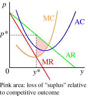
Consider a situation in which the market consists of a large number of buyers with various reservation prices, each of whom can either not buy the good or buy one unit of it, so that the demand curve represents the number of buyers whose reservation values exceed each possible price. Then the “surplus” in a trade between a buyer and the monopolist is the difference between the buyer's reservation price and the monopolist's cost of producing that unit---its MC. The part of this surplus that goes to the consumer is the difference between the reservation price and the price the monopolist charges, and the part that goes to the monopolist is the difference between the price it charges and its MC. Thus in this case the loss of "surplus" relative to the competitive equilibrium (in which price is equal to MC) is represented as the triangle in the following figure.

- Procedure for finding a monopolist's profit-maximizing output
-
- Find the output(s) for which MC(y*) = MR(y*).
- For each output you find, check to see whether the condition MC'(y*) ≥ MR'(y*) is satisfied.
- For each output that satisfies the first two conditions, check to see if profit is nonnegative.
- If there are any outputs satisfing these three conditions, the one that has the highest profit is the optimal output for the monopolist. (Most probably there is at most one output that satisfies the three conditions.) If there is no output that satisfies the three conditions the the optimal output for the monopolist is 0.
- Example
-
A monopolist has the cost function TC(y) = 200y + 15y2 and faces the demand function given by p = 1200 − 10y.
What output maximizes its profit? What is the profit-maximizing price? What is its maximal profit?
- We have TR(y) = (1200 − 10y)y = 1200y − 10y2, so
MR(y) = 1200 − 20y.AlsoMC(y) = 200 + 30y.Thus any output at which MR is equal to MC satisfies1200 − 20y = 200 + 30y,or50y = 1000, or y = 20.
- We have MR'(y) = −20 and MC'(y) = 30, so MC'(20) ≥ MR'(20).
- The price associated with y = 20 is p = 1200 − (10)(20) = 1000, so the firm's profit is
(1000)(20) − 200(20) − 15(20)2 = 20000 − 4000 − 6000 = 10000.Since this profit is positive, the optimal output for the monopolist is the output we have found, namely y* = 20. The price is 1000 and the monopolist's profit is 10000.
- We have TR(y) = (1200 − 10y)y = 1200y − 10y2, so
- Example
-
(A more complicated example to show the possibility of two outputs at which MR is equal to MC.)
A monopolist's cost function is TC(y) = (y/2500)(y − 100)2 + y, so that MC(y) = 3y2/2500 − 4y/25 + 5. It faces the inverse demand function P(y) = 4 − 4y/100. Find its output, the associated price, and its profit.
- For MR = MC we need
3y2/2500 − 4y/25 + 5 = 4 − 8y/100,or3y2/2500 − 8y/100 + 1 = 0,or3y2 − 200y + 2500 = 0,ory = [200 ± √(40,000 − 30,000)]/6 = [200 ± 100]/6 = 50 or 100/6.Thus there are two outputs at which MR is equal to MC: 50 and 100/6.
- We have
MR'(y) = −8/100 and MC'(y) = 6y/2500 − 4/25.We have MR'(50) = −8/100 = −0.08 and MC'(50) = −0.04, so that MC'(50) ≥ MR'(50). Also we have MR'(100/6) = −8/100 = −0.08 and MC'(100/6) = −0.12, so that MC'(100/6) < MR'(100/6). Hence the slope of MC is greater than the slope of MR only at y = 50.
- For y = 50 the price is P(50) = 4 − 200/100 = 2, so the firm's profit is (2)(50) − TC(50) = 100 − 100 = 0.
- For MR = MC we need
- Example: profit maximization and the effect of a lump sum tax
-
A monopolist's cost function is
It faces the demand function p = 300 − 5y. How much does the monopolist produce (as a function of F)? What is the price? What is the monopolist's profit?
TC(y) = 
0 if y = 0 100y + F if y > 0. - We have TR(y) = (300 − 5y)y, so MR(y) = 300 − 10y; MC(y) = 100. Thus for MC(y) = MR(y) we need y = 20.
- We have MR'(y) = −10 and MC'(y) = 0, so the condition MC'(y) ≥ MR'(y) is satisfied.
- For y = 20 the price is 300 − 5y = 200, so the profit is
TR(20) − TC(20) = (200)(20) − 2000 − F = 2000 − F.Thus the optimal output isIf the firm is in business then the price is p* = 200.
y* = 
0 if F > 2000 0 and 20 if F = 2000 20 if F < 2000.
Now suppose the firm has to pay a lump sum tax of T. Then its cost is
TC(y) = 100y + F + T if y > 0so that its marginal cost is exactly the same as before: MC(y) = 100. Thus the the output it chooses is not affected so long as the tax T isn't so large that the firm is better off shutting down---in this case, so long as 2000 − F − T > 0, or T < 2000 − F.Now suppose that the firm has to pay a fixed percentage tax on profit. Then it maximizes (1 − t)π(y) instead of π(y), where t is the tax rate. Since t is a constant, the solution of this problem is exactly the same as the solution of the original problem of maximizing π(y). Thus this tax has no effect on the monopolist's behavior.
- Example: the effect of an excise tax on monopoly behavior
-
Suppose the monopolist in the previous example has to pay a tax of $t for every unit it sells, rather than a lump sum tax.
- We now have TC(y) = 100y + F + ty, so MC(y) = 100 + t. (That is, MC shifts up by t.) Thus MR(y) = MC(y) when
300 − 10y = 100 + t,or y = 20 − t/10.
- As before, MR'(y) = −10 and MC'(y) = 0, so the condition MC'(y) ≥ MR'(y) is satisfied.
- The price is 300 − 5y = 300 − 100 − t/2 = 200 + t/2 and the profit is (200 + t/2)(20 − t/10) − [(100 + t)(20 − t/10) + F] = t2/20 − 20t + 2000 − F. If t is such that this profit is nonnegative then the output y = 2 − t/10 is optimal for the firm; if t is such that the profit is negative then the output 0 is optimal.
- We now have TC(y) = 100y + F + ty, so MC(y) = 100 + t. (That is, MC shifts up by t.) Thus MR(y) = MC(y) when
